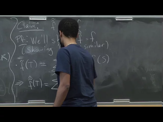
Harvard University · 1:26:14 · Watch on YouTube
Summary
A two-part lecture that closes the exponential-time algorithms in small space thread and opens the course's final topic, streaming and sketching. The first half derives the k-colorability inclusion–exclusion formula properly: it defines the zeta transform and Möbius inversion, proves they invert each other, and shows that the mysterious identity Σ_{S⊆V}(−1)^{|V−S|} f̂(S)^k > 0 is nothing but the Möbius inversion of f̂^k evaluated at V. Two ways to evaluate it are given — brute force in O*(3^n) time with polynomial space, and Yates's dynamic program in O*(2^n) time and space — settling k-colorability in roughly 2^n time. The second half sets up the turnstile streaming model, proves via an encoding argument that the distinct-elements problem F₀ admits no sublinear-space deterministic exact algorithm, maps out which of the four determinism/approximation variants survive, and closes with the idealized Flajolet–Martin min-hash estimator and its 1/ε²-copy averaging trick.
Topics
- Recap: inclusion–exclusion and the k-colorability formula
- Zeta transform and Möbius inversion
- Where the k-colorability formula comes from
- Brute force:
O*(3^n)time in polynomial space - Yates's algorithm:
O*(2^n)time and space - Applications, references, and finding an actual coloring
- The streaming model and the
F₀problem - Lower bound: no deterministic exact
F₀in sublinear space - The four variants: what is and isn't possible
- The idealized Flajolet–Martin algorithm
- Closing Q&A: point queries and other streaming problems
flowchart TD
    subgraph P1["Part 1 — inclusion–exclusion (0:00 – 47:45)"]
        A["Inclusion–exclusion fact<br/>Σ_{R⊆S⊆T}(−1)^{|T−S|} = [R=T]"] --> B["ζ and μ are inverses:<br/>(f̂)~ = (f̃)^ = f"]
        B --> C["ĝ(S) = f̂(S)^k<br/>(counting argument)"]
        C --> D["k-colorable ⟺<br/>Σ_S (−1)^{|V−S|} f̂(S)^k > 0"]
        D --> E["Brute force:<br/>3^n time, poly space"]
        D --> F["Yates DP:<br/>2^n time and space"]
    end
    subgraph P2["Part 2 — streaming (47:45 – end)"]
        G["Turnstile model:<br/>update (i,v): x_i += v"] --> H["F₀ = support size"]
        H --> I["Encoding argument ⇒<br/>deterministic exact needs Ω(min(n,m))"]
        I --> J["Only randomized + approximate<br/>is possible sublinearly"]
        J --> K["Flajolet–Martin:<br/>Z = min h(i), output 1/Z − 1"]
        K --> L["Average 1/ε² copies<br/>⇒ (1 ± ε) guarantee"]
    end
    P1 -.->|"course pivots to<br/>the lecturer's own area"| P2
Key takeaways
- The k-colorability formula is a derivation, not a trick:
g(V) = (f̂^k)~(V), becauseĝ(S) = f̂(S)^k— both sides count orderedk-tuples of non-empty independent sets contained inS— and Möbius inversion undoes the zeta transform20:26,23:03,23:34. - Overlap doesn't matter for coloring: a union of
kpossibly-overlapping non-empty independent sets can always be turned into a disjoint one by keeping each vertex in only the first set it appeared in19:12,19:35. - Inclusion–exclusion buys space, not time, at first: brute force evaluates the formula in
O*(3^n)time with poly(n) space — matching last lecture's DP in time while dropping its2^nspace — because eachf̂(S)is folded into a running sum and discarded26:42,27:47,28:05. - Yates's algorithm decides k-colorability in
O*(2^n): the recurrenceG(i,S) = G(i−1,S) + [i∈S]·G(i−1,S−i)with baseG(0,S) = f(S)hasn·2^nstates andO(1)work each, so time ≈ space32:43,34:03,40:20. - Best known poly-space bound is
O*(2.2461^n)(Björklund–Husfeldt, FOCS '06); reaching ~2^ntime in polynomial space is an open problem6:40,7:16. - Decision implies construction for free: a black-box reduction of a couple of paragraphs turns any
2^n-time chromatic-number algorithm into one that outputs an actualk-coloring in roughly the same time44:20,45:25. - Deterministic exact
F₀needsΩ(min(n,m))bits (AMS '96/'99): a space-Salgorithm would compress everyn-bit string toSbits — Alice streams the 1-indices and ships the memory image, Bob re-insertsi = 1..nand readsx_ioff whether the count moves — contradicting pigeonhole unlessS ≥ n56:47,59:27,1:04:43. - Three of the four
F₀variants are impossible sublinearly: deterministic-exact, deterministic-approximate (for any constant factor, not just 1%), and randomized-exact all fail; only randomized + approximate works, via Flajolet–Martin (JCSS '85)1:06:56,1:07:20,1:08:16. - Flajolet–Martin's estimator is one number:
Z = min_i h(i)over the stream, output1/Z − 1, justified byPr[Z > x] = (1−x)^{F₀}givingE[Z] = 1/(F₀+1)(andE[Z²] = 2/((F₀+1)(F₀+2)))1:13:31,1:19:38,1:20:00. - Averaging
R = 1/ε²independent copies converts constant error into1 ± ε: the mean is unchanged, the variance drops by a factorR, exactly cancelling theε²in Chebyshev's bound1:15:13,1:21:58. - Point queries behave differently from
F₀: deterministic approximate becomes possible there (error± ε‖x‖₁), at space≈ 1/ε²deterministically and≈ 1/εrandomized — but it cannot be recycled into a deterministicF₀approximation, since a true zero and anε‖x‖₁-sized value are indistinguishable1:23:33,1:24:20,1:25:38.