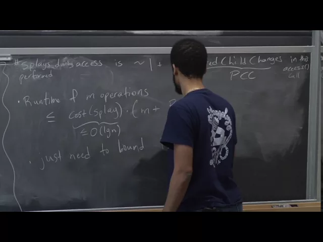
Harvard University · 1:26:46 · Watch on YouTube
Summary
A lecture in two halves. First, Jelani Nelson completes the amortized analysis of link-cut trees, introducing the heavy-light decomposition purely as an accounting device: every operation's cost is charged to preferred child changes, those are charged to light preferred edge creations, and each root-to-vertex path carries at most log n light edges — yielding O(m log² n + n log n) for m operations, with the improvement to O(m log n) (same structure, sharper splay analysis) left to the problem set. Second, he opens min-cost max flow: costs in the residual graph negate on reverse edges, the problem is interreducible with min-cost circulation, and the naive negative-cycle canceling algorithm is correct — via a decomposition of any circulation into at most m cycles — but only pseudo-polynomial at O(mn · mUC). The fix is the price function / reduced cost machinery: a circulation is optimal iff some price function makes all reduced costs non-negative, which in the unit-capacity, non-negative-cost case makes successive shortest paths with Dijkstra valid and gives O(mn + n² log n).
Topics
- Logistics and lecture roadmap
- Link-cut tree operations: recap of
access,cut,link - Reducing the runtime to preferred child changes
- The heavy-light decomposition (analysis tool)
- Bounding
PCCby light preferred child creations - Bounding
LPCCacrossaccess,link,cut— and the final bound - Augmented BSTs inside aux trees
- Min-cost max flow: the problem and residual costs
- Min-cost circulation and its equivalence with min-cost max flow
- Negative-cycle canceling for min-cost circulation
- Price functions, reduced costs, and the optimality characterization
- Faster min-cost max flow: successive shortest paths
flowchart TD
    subgraph LCT["Part 1 — Link-cut tree analysis (topics 2–7)"]
        T1["runtime ≤ splay cost × (m + PCC)"] --> T2["PCC ≤ 2·LPCC + m + n<br/>(heavy-light charging)"]
        T2 --> T3["LPCC = O(m log n)<br/>(≤ log n light edges per root path)"]
        T3 --> T4["O(m log² n + n log n)"]
        T4 -.->|"pset 8: sharper splay analysis"| T5["O(m log n)"]
    end
    subgraph MCF["Part 2 — Min-cost max flow (topics 8–12)"]
        F1["Min-cost max flow<br/>reverse residual edge has cost −c(e)"] <-->|"reduce both ways"| F2["Min-cost circulation"]
        F2 --> F3["Cancel negative cycles<br/>(Bellman–Ford / Goldberg '95)"]
        F3 --> F4["Correct, but pseudo-polynomial:<br/>O(mn · mUC)"]
        F4 --> F5["Price function p:<br/>c_p(uv) = c(uv) + p(u) − p(v)<br/>optimal ⟺ all c_p ≥ 0"]
        F5 --> F6["Unit capacity, non-negative costs:<br/>successive shortest paths + Dijkstra<br/>O(mn + n² log n)"]
    end
    LCT -.->|"link-cut trees existed to<br/>speed up blocking flow"| MCF
Key takeaways
mlink-cut tree operations run inO(m log² n + n log n)amortized; then log nterm is harmless in blocking-flow use, wherem ≥ nandm log² ndominates42:15,43:23.log² nimproves tolog nwith no change to the data structure — only a better amortized analysis of the splay trees, via the lecture-7 access lemma with the right weight function1:35,2:09,43:39.- The whole analysis reduces to
PCC ≤ 2·LPCC + m + n: light creations are counted directly, heavy creations at a childless parent are charged one dollar to the last access (+m,+n), and heavy creations at a parent that already had a preferred child must destroy a light preferred edge — since a vertex has at most one heavy child — giving the factor 216:15,24:37,25:29. LPCC = O(m log n)because a root-to-vertex path contains at mostlog nlight edges (subtree size ≤n, halved at each light edge), andaccesschanges only preferred-ness, never light/heavy27:46,29:26,30:30.linkandcutare essentially free beyond their accesses: edges that get lighter aren't preferred, and heavy creations are not counted at all —cutadds onlyO(log n)more along one root-to-leaf path35:15,35:40,40:22.- Min-cost max flow and min-cost circulation reduce to each other; the clean one-call direction is find any max flow ignoring costs, then find a min-cost circulation in its residual graph and add it back — valid because the difference of two equal-value
s–tflows is a circulation53:29,1:00:24,1:01:10. - Negative-cycle canceling is correct but pseudo-polynomial:
O(mn)per Bellman–Ford iteration (orO(m√n log C)by Goldberg '95) times at mostmUCiterations — explicitly "the Ford–Fulkerson of min-cost circulation"1:03:58,1:10:50. - Correctness rests on cycle decomposition: any circulation splits into at most
mcycles (extract a cycle at its minimum capacity, saturating ≥ 1 edge each time), so a negative circulation must contain a negative cycle1:07:58,1:08:56. - Optimality characterization:
fis a min-cost circulation iff a price functionpexists withc_p(uv) = c(uv) + p(u) − p(v) ≥ 0everywhere — the prices cancel around cycles, so cycle costs are unchanged; the witness isp(u) =shortest-path distance from a new zero-cost super-source, well defined exactly because no negative cycles exist1:13:23,1:14:08,1:15:29. - Unit capacities with non-negative costs:
O(mn + n² log n)by successive shortest paths — ≤niterations of Dijkstra with Fibonacci heaps. Dijkstra stays legal because every edge on a shortest path has reduced cost exactly 0, so the saturated edge's reverse enters the residual graph at−0 = 01:19:43,1:22:52,1:23:41. - Negative cycles are handled by preprocessing, not by a new algorithm: saturate every negative edge outright, then repair the resulting imbalances with a new source/sink whose capacities equal the exact excesses — leaving a non-negative-cost instance
1:24:57,1:25:19,1:25:45.