Harvard University · 1:26:44 · Watch on YouTube
Summary
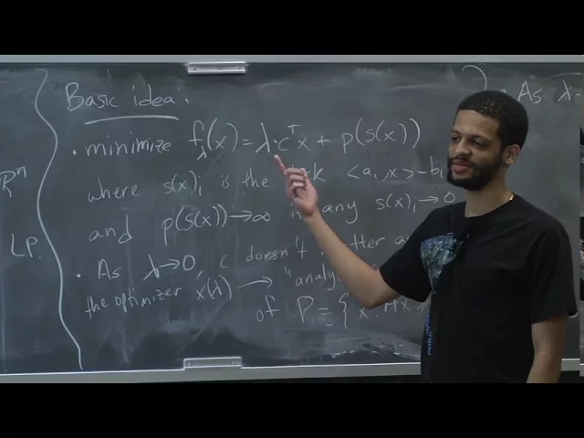
A university lecture on the interior point method (IPM) for linear programming. The first half sets up the method: replace min cᵀx s.t. Ax ≥ b by the penalized objective f_λ(x) = λ·cᵀx − Σ log s(x)ᵢ, follow the resulting central path from the analytic center of the feasible region toward the optimal vertex as λ grows, and prove the suboptimality bound cᵀx_λ − cᵀx* ≤ m/λ that says when to stop. Combining that with a (1 + 1/√m) step size for λ yields the classical √m·L iteration count, and the lecture places it against Karmarkar's O(mL), Renegar's O(√m·L), and the then-brand-new Lee–Sidford Õ(√rank(A)·L). The second half is an optimization digression — oracles, Hessian bounds under the Loewner ordering, and a full derivation and convergence proof of gradient descent — as the warm-up for Newton's method, the second-order method that will actually drive each IPM iteration in the next lecture.
flowchart TD
    subgraph P1["Part 1 — Interior point method"]
        A["LP setup + log barrier<br/>(01)"] --> B["5-step algorithm outline<br/>(02)"]
        B --> C["Stopping rule: c'x_lambda - c'x* <= m/lambda<br/>(03)"]
        C --> D["sqrt(m)*L iterations + history<br/>(04)"]
        D --> E["Central path / path-following<br/>(05)"]
    end
    subgraph P2["Part 2 — Optimization background"]
        F["Oracles, Hessian bounds, Loewner order<br/>(06)"] --> G["Gradient descent: derivation + rate<br/>(07)"]
        G --> H["Acceleration; Newton's method preview<br/>(08)"]
    end
    E --> F
    H -.->|"seeds each IPM iteration"| B
Topics
- LP setup and the barrier-function idea
- The five-step algorithm outline
- Stopping criterion: the
m/λsuboptimality bound - Iteration count and the history of IPM bounds
- The central path and path-following IPMs
- Optimization background: oracles, Hessian bounds, Loewner ordering
- Gradient descent: where it comes from and how fast it converges
- Acceleration, and what comes next (Newton's method)
Also in this folder: transcript.md, the verbatim timestamped transcript.
Key takeaways
- The central suboptimality bound is
cᵀx_λ − cᵀx* ≤ m/λ, proved from the single fact that slack vectors are non-negative, after setting∇f_λ(x_λ) = 0and dotting withx_λ − x*(29:42,29:19). - Stopping is therefore a threshold on λ: run until
λ ≥ m/ε ≈ m·exp(CL)withεexponentially small in the precisionL, at which point the iterate rounds to the exact optimal vertex (30:30,30:52,19:32). - The step
λk+1 = (1 + 1/√m)·λkgives√m·(L + log m) ≈ √m·Literations, because√msteps multiplyλby a constant factor andlogof theλ₀-to-target ratio isO(L + log m)(31:41,34:20,35:28). - Historical progression of IPM iteration bounds:
O(mL)(Karmarkar, Combinatorica 1984) →O(√m·L)(Renegar, 1988) →Õ(√rank(A)·L)(Lee and Sidford, FOCS, announced about a week before this lecture) (35:28,36:57). - Per iteration the algorithm never solves
f_λexactly — it computes approximate minimizers, at a cost of a constant number of linear-system solves onn × nmatrices (38:52,39:08). - Gradient descent contracts error by
1 − μ/Lper step, givingO(L/μ)iterations to halve the error andO((L/μ)·log(1/ε))to go fromδtoεδ; Nesterov's accelerated gradient descent (Soviet Math 1983) does it inO(√(L/μ)), though the distinction is irrelevant for IPM since its control parameters are constants (1:15:22,1:20:03,1:21:08,1:22:02). - IPM will use Newton's method, not gradient descent, because it needs to explicitly compute the Hessian rather than merely bound it (
1:24:14,57:44).