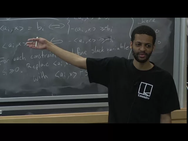
Harvard University · 1:26:13 · Watch on YouTube
Summary
After many lectures treating linear programming as a black box, this lecture finally opens the box and develops the Simplex algorithm from scratch. It builds the machinery in order: reducing any LP to standard form (min cᵀx, Ax = b, x ≥ 0), defining a vertex of the polytope, showing how to obtain a starting vertex by running Simplex on an auxiliary LP, proving that a bounded LP attains its optimum at a vertex, and proving that x is a vertex iff the columns of A on its support are linearly independent. That characterization turns vertices into bases — sets of m independent columns — which lets the LP be rewritten around any base so that the objective becomes a constant plus reduced costs c̃_N on the non-basic variables. Simplex then reads off as: halt when c̃_N ≥ 0, otherwise increase a negative-reduced-cost variable and pivot; the lecture closes on Bland's Rule for avoiding cycling and on the gap between Simplex's exponential worst case and its practical speed.
Content type: educational video — a university lecture (theorem/proof style, with live Q&A from students).
flowchart TD
    A[Any LP] --> B[Standard form<br/>min cᵀx, Ax=b, x≥0]
    B --> C[Geometry: polytope P<br/>vertex = no y with x±y ∈ P]
    C --> D[Auxiliary LP<br/>gives a starting vertex]
    C --> E[Bounded LP ⟹<br/>optimum at a vertex]
    C --> F[Vertex ⟺ independent<br/>columns of A on supp x]
    F --> G[Bases of size m<br/>x_B = A_B⁻¹ b]
    G --> H[Rewrite LP → reduced costs c̃_N]
    D --> I[SIMPLEX]
    E --> I
    H --> I
    I --> J[Pivoting rules · Bland 1977]
    J --> K[Exponential worst case<br/>vs. ellipsoid / interior point]
Topics
- Course logistics and lecture roadmap — project proposal deadline, and the three-part plan: Simplex, strong duality, ellipsoid.
- Putting any LP into standard form — the four reductions (max→min,
=→two≥,≤→≥, slack variables) and whyn ≥ m. - The geometric picture and the definition of a vertex — Simplex as a greedy walk over vertices (Dantzig, 1947) and the formal definition of a vertex.
- Getting an initial vertex — why feasibility ≡ optimization, the bit-precision bound, and the auxiliary LP
min twithAx = (1−t)b. - Vertices attain the optimum — the bounded-LP claim, its two-case proof,
t* = min(−x_j/y_j), and the two corollaries. - Vertices ⟺ linearly independent columns — the support submatrix
A_{B(x)}, both contrapositives, and|B(x)| ≤ m. - Bases and rewriting the LP around a vertex —
x_B = A_B⁻¹ b, base padding, and the reduced-cost form of the objective. - The Simplex algorithm and pivoting rules — the halting condition
c̃_N ≥ 0, degenerate bases, cycling, and Bland's Rule. - Simplex in practice vs. polynomial-time LP — exponential worst case, ellipsoid, interior-point methods.
Key takeaways
- Every LP can be forced into standard form
min cᵀx, Ax = b, x ≥ 0using four mechanical reductions, and the slack-variable step automatically guaranteesn ≥ m(at least as many variables as constraints)9:07,9:26,9:43. - A bounded LP always attains its optimum at a vertex: for any feasible
xthere is a vertexx′withcᵀx′ ≤ cᵀx, proved by repeatedly stepping along a kernel directiony— a step that creates a new zero coordinate and can therefore recur at mostntimes, while the alternative case would force the LP to be unbounded27:38,41:49,44:11. - Corollary: a non-empty standard-form polytope always has a vertex — apply the result with the trivial objective
min 0ᵀx. This fails outside standard form, where a feasible region can be a vertex-free strip48:15,49:22,49:55. xis a vertex iff the columns ofAon{ j : x_j > 0 }are linearly independent, which caps the support at|B(x)| ≤ mand makes a vertex fully recoverable from its base by solvingx_B = A_B⁻¹ b. Combined with then choose mbound on the number of vertices, this is what bounds the precision needed to write down OPT51:04,52:53,1:05:33,17:59.- Simplex's stopping rule is
c̃_N ≥ 0: rewriting the LP in the current base turns the objective into a constantc_Bᵀ A_B⁻¹ bplus reduced costs on non-basic variables, so a negativec̃_jis exactly a direction of improvement1:13:08,1:15:22,1:16:34. - Naive pivoting can cycle forever; Bland's Rule (Bland, Math. of OR, 1977) provably cannot. Practitioners nonetheless still use rules known to cycle, judging cycling to be contrived in practice
1:21:58,1:22:27,1:23:55. - No known pivoting rule is even sub-exponential, let alone polynomial — so Simplex is theoretically slow yet practically dominant; ellipsoid was the first polynomial-time LP algorithm but is impractical, while interior-point methods are both polynomial and fast
1:24:46,1:25:25,1:25:50. - Strong duality comes free from Simplex: at the halting condition one can directly read off a dual feasible solution achieving the same cost as the primal (proof deferred to the next lecture)
2:26,1:23:26.